EUFISICA · José Gonçalves

Space explorationPhysics explained

The Physics of Rockets

From Newton's laws and the rocket equation to orbital mechanics and the future of space exploration.

How can a vehicle weighing hundreds of tonnes accelerate through Earth's atmosphere, reach orbit, and travel through deep space? The answer combines conservation of momentum, thermodynamics, fluid dynamics, and orbital mechanics. In this illustrated guide, we derive the fundamental equations, examine real-world scales, and use mathematical models to investigate rocket performance.

Circular speed · 400 km altitude

7.67 km/s

Approximately 27,600 km/h

Escape speed · Earth's surface

11.2 km/s

Ideal, unpowered escape condition

01 / FUNDAMENTALSWhy do rockets work in a vacuum?

Newton's third law describes a fundamental aspect of rocket propulsion: when a rocket accelerates exhaust gases backwards, the gases transfer momentum to the rocket in the opposite direction. The rocket does not push against air. Because it carries both fuel and oxidizer (for chemical propulsion), it can generate thrust in a vacuum.

For a rocket engine carrying its own propellants, the thrust is

F_T = ṁv_e + (p_e − p_a)A_e

Symbol	Physical meaning	SI unit
FT	Engine thrust	N
ṁ	Propellant mass flow rate	kg/s
ve	Exhaust velocity relative to engine	m/s
pe, pa	Exit and ambient pressure	Pa
Ae	Nozzle exit area	m²

The first term represents momentum thrust; the second is pressure thrust. A nozzle converts thermal energy into directed exhaust kinetic energy. Its geometry influences exhaust velocity and pressure, and therefore engine performance.

Worked example. For ṁ = 250 kg/s and v_e = 3,000 m/s, assuming zero pressure contribution, F_T = (250)(3,000) = 750,000 N = 750 kN.

02 / ASCENTForces acting on a rising rocket

During vertical powered ascent, the major forces are thrust upwards, gravity downwards, and aerodynamic drag opposite the velocity. Newton's second law gives a simplified instantaneous model:

ma = F_T − mg − D

A vertical launch requires thrust to exceed weight at the moment of liftoff:

TWR = F_Tmg > 1

For a 50,000 kg rocket producing 750 kN, its initial thrust-to-weight ratio is approximately 1.53, and its initial acceleration without drag is 5.19 m/s². As propellant is consumed, the mass decreases, so acceleration can rise even if thrust stays constant.

03 / VARIABLE-MASS MECHANICSThe Tsiolkovsky rocket equation

The central challenge of rocket flight is that the rocket becomes lighter while it burns propellant. Conservation of momentum yields, for an ideal rocket with constant effective exhaust speed and no external forces:

m dv = −v_eq dm

Separate variables and integrate from initial mass m₀ to final mass m_f:

∫ dv = −v_eq ∫ (dm / m)

Δv = v_eq ln(m₀ / m_f)

Since the effective exhaust speed is v_eq = I_spg₀, with g₀ = 9.80665 m/s²:

Δv = I_spg₀ ln(MR)

Here MR = m₀/m_f is the mass ratio, and I_sp is the specific impulse in seconds. Because the equation is logarithmic, much larger propellant fractions are necessary to achieve additional velocity increments.

Model: ideal delta-v

Figure 1. Ideal velocity increment versus initial-to-final mass ratio. Curves are calculated directly from the Tsiolkovsky equation; gravity and aerodynamic losses are excluded.

*Assumes the mass lost is solely expelled propellant; final mass includes dry structure and payload.

04 / PROPULSIONSpecific impulse and engine performance

Specific impulse describes how effectively a propulsion system uses its propellant. It is defined using standard gravity (not the local gravitational acceleration):

I_sp = F_Tṁg₀

Higher I_sp generally means more total impulse per unit propellant weight. However, a high-I_sp engine does not necessarily have high thrust: chemical launch engines and electric spacecraft thrusters serve very different missions.

Illustrative Isp	Equivalent exhaust velocity
250 s	2.45 km/s
300 s	2.94 km/s
350 s	3.43 km/s
450 s	4.41 km/s

These are calculated examples, not measured performance data for specific engines.

05 / VEHICLE DESIGNWhy rockets have multiple stages

Carrying empty tanks and spent engines requires extra propellant. In a multistage launcher, exhausted stages are released so the remaining vehicle accelerates with less inert mass. The ideal velocity increments of the individual stages add:

Δv_total = Σ [I_sp,i g₀ ln(m_0,i/m_f,i)]

Figure 2. Simplified conceptual illustration of staging and spacecraft deployment. Not to scale.

Actual mission design also accounts for separation events, structural limits, guidance, and the mass of carried upper stages and payload.

06 / ORBITAL PHYSICSReaching space is not the same as reaching orbit

To remain in a circular orbit, a spacecraft needs sufficient tangential velocity to continuously fall around Earth. Gravity provides the required centripetal acceleration:

GMmr² = mv²r

v_orb = √(GM / r) = √(μ / (R + h))

Here μ = GM is Earth's standard gravitational parameter, R is the mean Earth radius, and h is altitude above that idealized spherical Earth.

Model: orbital speed and altitude

Figure 3. Ideal circular-orbit speed against altitude, using μ = 398,600.4418 km³/s² and R = 6,371 km. Atmospheric drag, Earth's oblateness, and orbital perturbations are neglected.

At 400 km altitude, the ideal circular-orbit speed is about 7.67 km/s, or 27,600 km/h. A launch vehicle needs a larger total delta-v budget because of gravity losses, aerodynamic drag, steering and mission constraints.

07 / ENERGYEscape velocity

Escape speed comes from conservation of mechanical energy. At the minimum escape condition, an unpowered object reaches an infinite distance from Earth with zero remaining speed:

12mv² − GMmR = 0

v_esc = √(2GM / R)

At the Earth's surface, the result is approximately 11.2 km/s. This is not a required instantaneous liftoff speed: a powered spacecraft can gain energy over time through continuous or repeated engine burns.

08 / ATMOSPHERIC FLIGHTDrag, dynamic pressure and Max-Q

Atmospheric drag depends on air density, the square of air-relative speed, reference area, and drag coefficient:

D = ½ρv²C_DA

Dynamic pressure is q = ½ρv². Early in ascent, speed increases while atmospheric density decreases with altitude. Their competing effects often produce a maximum dynamic pressure known as Max-Q. Rockets may throttle their engines during high-load portions of the climb to protect the vehicle.

09 / GUIDANCEThe gravity turn: from vertical flight to orbit

Rockets initially climb close to vertically to clear the launch facility and dense lower atmosphere. They then tilt and build the horizontal speed required for orbit. A carefully planned gravity turn can reduce the steering effort needed during much of the ascent.

01Liftoff

02Pitch over

03Max-Q

04Stage separation

05Orbit insertion

Exact timing and trajectory depend on rocket design, launch site, payload and target orbit; this sequence is conceptual rather than a universal flight schedule.

10 / TECHNOLOGYChemical versus electric propulsion

Chemical rockets

Propellants release chemical energy and produce large exhaust mass flow rates, enabling high thrust. They dominate launches from planetary surfaces and are also used for major orbital manoeuvres.

Electric propulsion

Ion and Hall-effect thrusters use electrical energy to accelerate charged particles. They commonly deliver low thrust but much higher specific impulse, making them valuable for long-duration in-space missions.

11 / DATAKey Earth and orbit reference values

Quantity	Approximate value	Context
Mean Earth radius	6,371 km	Spherical model
Earth gravitational parameter	398,600 km³/s²	Standard value, rounded
Standard gravity	9.80665 m/s²	Conventional reference
Circular speed at 400 km	7.67 km/s	Ideal two-body orbit
Orbital period at 400 km	92.4 min	Ideal two-body orbit
Escape speed at surface	11.2 km/s	No atmospheric resistance

12 / CONCLUSIONPhysics makes space exploration possible

Rocket engineering unites principles that students encounter throughout physics: momentum conservation explains thrust, variable-mass dynamics determines available delta-v, thermodynamics and fluid dynamics govern the engine, and gravitation sets the conditions for orbital flight and escape.

Rocket science is not magic: it is physics in action. Every successful mission is a practical demonstration of those laws — and of the engineering required to use them.

REFERENCESSources and further reading

1. NASA Glenn Research Center. (n.d.). Rocket thrust equation. NASA Glenn.
2. NASA Glenn Research Center. (n.d.). Ideal rocket equation. NASA Glenn.
3. NASA Glenn Research Center. (n.d.). Specific impulse. NASA Glenn.
4. NASA Glenn Research Center. (n.d.). Guide to rockets. NASA Glenn.
5. Sutton, G. P., & Biblarz, O. (2017). Rocket propulsion elements (9th ed.). Wiley.
6. Curtis, H. D. (2020). Orbital mechanics for engineering students (4th ed.). Butterworth-Heinemann.

EUFISICA · José Gonçalves
Physics · Science education · Space exploration

Houston we have a problem... in Mars

This is a theoretical problem on a Mars habitat and the astronauts have to move it from the planet.
Check the full reading:

Physics of Superheroes

In the past, I posted about the Physics of Spiderman 3, Superman. 

Today, I present in this blog a paper about Physics and Superheroes.

The Standard Model

Standard Model - Source: Wikipedia

 The Standard Model of particle physics is the theoretical framework that describes the fundamental building blocks of the universe and the forces through which they interact. It is one of the most successful and rigorously tested theories in modern physics.

Here is a breakdown of how the universe is put together according to the Standard Model.

1. The Building Blocks: Matter Particles (Fermions)

All tangible matter in the universe is made up of particles called fermions, which have half-integer spin (e.g., 1/2). These are divided into two main categories, each split into three "generations" of increasing mass.

Quarks

Quarks are heavy particles that experience the strong nuclear force. They combine to form composite particles called hadrons (like protons and neutrons).

• Generation 1: Up (u), Down (d) — These make up ordinary stable matter.

• Generation 2: Charm (c), Strange (s)

• Generation 3: Top (t), Bottom (b)

Leptons

Leptons do not feel the strong nuclear force.

• Generation 1: Electron (e^-), Electron Neutrino (ν_e)

• Generation 2: Muon (μ), Muon Neutrino (ν_μ)

• Generation 3: Tau (τ), Tau Neutrino (ν_τ)

Note: For every matter particle, there is a corresponding antimatter particle with the same mass but opposite electric charge (e.g., the positron is the antielectron).

2. The Messengers: Force Carriers (Gauge Bosons)

Particles interact by exchanging force-carrier particles called gauge bosons, which have integer spin (e.g., 1). The Standard Model accounts for three of the four fundamental forces of nature:

Force	Description	Gauge Boson (Carrier)	Mass / Range
Electromagnetism	Governs atomic structure, light, and chemical reactions.	Photon (γ)	Massless / Infinite
Strong Nuclear Force	Binds quarks inside protons/neutrons and holds atomic nuclei together.	Gluon ($g$)	Massless / Short-range
Weak Nuclear Force	Responsible for radioactive decay (like beta decay) and initiating solar fusion.	W+ / W- and Z0 Bosons	Very heavy / Ultra short-range

3. The Mass Giver: The Higgs Boson

The Higgs Boson (H) is a scalar boson (spin 0) associated with the Higgs field, which permeates the entire universe.

• Mechanism: As fundamental particles move through this field, they interact with it. The strength of this interaction determines the particle's inertial mass.

• Particles like the top quark interact strongly and are very heavy; photons do not interact with it at all and remain massless.

• Its discovery at CERN's Large Hadron Collider (LHC) in 2012 was the final piece confirming the Standard Model's framework.

What the Standard Model Left Out

While incredibly robust, the Standard Model is known to be an incomplete theory of nature because it fails to explain a few massive cosmological puzzles:

• Gravity: It does not include general relativity. The hypothetical carrier of gravity, the graviton, has not been incorporated mathematically into the quantum framework.

• Dark Matter & Dark Energy: The model only accounts for about 5% of the energy-mass composition of the observable universe. The remaining 95% is completely unaccounted for.

• Neutrino Mass: In the original mathematical formulation of the Standard Model, neutrinos are massless. However, oscillation experiments have proved they possess tiny, non-zero masses.

• Matter-Antimatter Asymmetry: It doesn't fully explain why the universe today is overwhelmingly made of matter, even though the Big Bang should have produced equal amounts of matter and antimatter.

Physics and Cristiano Ronaldo

 

Jupiter Notebook File (PT)

Eggnaut challenge

 

Eggnaut protection created with Gemini

One of the students’ favorite challenges is the Eggnaut experiment. In this activity, they use the physics learned in secondary school along with engineering, management, economics, and other skills to create a cost-effective solution to protect the egg.

You can check the "Jupiter" book in python here: Simulations/eggnaut.ipynb at main · eufisica/Simulations

Jupiter code about the Hellium Chewing Gum

This post (from 2010!) explained the Physics behind a fake video.

There wasn't AI to  try to explain the phenomenom. But we have it today. So I took all the Physics and put it in a Jupiter file available here: Simulations/helium gum exp.ipynb at main · eufisica/Simulations

By the way, the new website is ready and available here: EUFISICA.

The Scale of the Universe

Scales in the Universe - Created with Gemini AI

 The scale of the universe is so vast that our everyday units of measurement completely break down. To comprehend it, physicists and astronomers look at the universe across orders of magnitude, moving from the microscopic quantum realm up to the edge of everything we can see.

1. The Microscopic Limit: Quantum Scale

Before looking outward, understanding the absolute smallest limits of space helps frame the true extremes of scale.

• The Planck Length (1.6 x 10^-35 m): The theoretical smallest possible distance in physics. Below this scale, the traditional concept of space and time ceases to exist.

• Subatomic Particles (10^-18 m to 10^-15 m): Quarks and electrons have no measurable size, but a proton or neutron spans about 1 femtometer (10^-15 m.

• The Atom (10^-10 m): An atom is roughly 0.1 nanometers across. If an atom were magnified to the size of a massive sports stadium, its nucleus would only be the size of a marble in the center.

2. The Human and Planetary Scale

Moving up to lengths we can physically perceive, objects grow exponentially as we exit Earth's atmosphere.

• Humans (10⁰ m): Positioned roughly in the middle of the cosmic scale between the Planck length and the observable universe.

• Earth (1.27 x 10⁷ m): With a diameter of roughly 12,742 km.

• The Sun (1.39 x 10⁹ m): Approximately 109 times the diameter of Earth. You could fit about 1.3 million Earths inside it.

3. The Cosmic Scale: Light-Years and Parsecs

Once we leave the Solar System, the meter becomes too small to be practical. Instead, we measure distances by how far light travels in a year (one light-year, or ~ 9.46 x 10¹⁸ m).

• Solar System & Neighborhood: The distance from Earth to the Sun is 1 Astronomical Unit (a.u.)}. The nearest star system to us, Alpha Centauri, is about 4.37 light-years away.

• The Milky Way (10²¹ m): Our home galaxy is a spiral disk roughly 100,000 light-years across, containing hundreds of billions of stars.

• The Local Group & Superclusters (10²³ m): The Milky Way belongs to a small cluster called the Local Group (spanning 10 million light-years), which itself is a tiny branch of the massive Laniakea Supercluster, home to over 100,000 galaxies.

4. The Observable Universe

The observable universe is a spherical region centered on Earth, encompassing everything we can theoretically detect because its light has had time to reach us since the Big Bang.

• The Diameter: While the universe is about 13.8 billion years old, the expansion of space means the edge of the observable universe has stretched farther away. Its current diameter is estimated to be roughly 93 billion light-years (8.8 x 10²⁶ m).

• The Content: It contains up to 2 trillion galaxies and an estimated 10²⁴ stars—more stars than there are grains of sand on all of Earth's beaches.

• Beyond the Observable: Because cosmic inflation expanded space faster than the speed of light during the earliest moments of the Big Bang, the entire universe is likely far larger than what we can observe—and it may well be infinite.

Would you like to explore a specific realm of this scale further, such as the math behind cosmological expansion, or how we measure these immense distances using standard candles?

How Big is The Universe?

This video provides an excellent visual journey zooming out from Earth to the edges of the observable universe to help contextualize these massive cosmic distances.

Take a look in this website: http://scaleofuniverse.com/

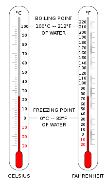
Build your thermo scale

Do you want to know more about thermometers?

Well check this website, choose your scale and see how it's the formula (see the image below).

Update (12-12-2021): You need to download the file (right click with your mouse and select "save link as...") and you can run in your computer (you need Adobe Flash Player installed in your computer).

Thermometers

Developed during the 16th and 17th centuries, a thermometer (from the Greek θερμός (thermos) meaning "warm" and meter, "to measure") is a device that measures temperature or temperature gradient using a variety of different principles. A thermometer has two important elements: the temperature sensor (e.g. the bulb on a mercury thermometer) in which some physical change occurs with temperature, plus some means of converting this physical change into a numerical value (e.g. the scale on a mercury thermometer).

Read more in Wikipedia.

Farenheit Scale

Fahrenheit is the temperature scale proposed in 1724 by, and named after, the German physicist Daniel Gabriel Fahrenheit (1686–1736). Within this scale, the freezing of water into ice is defined at 32 degrees, while the boiling point of water is defined to be 212 degrees. The temperature scale was replaced by the Celsius scale in most countries during the mid to late 20th century, but it remains the official scale of the United States, Cayman Islands and Belize.

Read more in Wikipedia.

Celsius Scale

Celsius is a scale and unit of measurement for temperature. It is named after the Swedish astronomer Anders Celsius (1701–1744), who developed a similar temperature scale two years before his death. The degree Celsius (°C) can refer to a specific temperature on the Celsius scale as well as a unit to indicate a temperature interval, a difference between two temperatures or an uncertainty. The unit was known until 1948 as "centigrade" from the Latin "centum" translated as 100 and "gradus" translated as "steps".

Credit: uoregon.edu

From 1744 until 1954, 0 °C was defined as the freezing point of water and 100 °C was defined as the boiling point of water, both at a pressure of one standard atmosphere with mercury being the working material. Although these defining correlations are commonly taught in schools today, by international agreement the unit "degree Celsius" and the Celsius scale are currently defined by two different temperatures: absolute zero, and the triple point of VSMOW (specially-purified water). This definition also precisely relates the Celsius scale to the Kelvin scale, which defines the SI base unit of thermodynamic temperature with symbol K. Absolute zero, the lowest temperature possible at which matter reaches minimum entropy, is defined as being precisely 0 K and −273.15 °C. The temperature of the triple point of water is defined as precisely 273.16 K and 0.01 °C.

This definition fixes the magnitude of both the degree Celsius and the kelvin as precisely 1 part in 273.16 (approximately 0.00366) of the difference between absolute zero and the triple point of water. Thus, it sets the magnitude of one degree Celsius and that of one kelvin as exactly the same. Additionally, it establishes the difference between the two scales' null points as being precisely 273.15 degrees Celsius (−273.15 °C = 0 K and 0 °C = 273.15 K).

Read more in Wikipedia.

Rankine Scale

Rankine is a thermodynamic (absolute) temperature scale named after the Glasgow University engineer and physicistWilliam John Macquorn Rankine, who proposed it in 1859. (The Kelvin scale was first proposed in 1848.)

The symbol for degrees Rankine is R^[1] (or Ra if necessary to distinguish it from the Rømer and Réaumur scales). Zero on both the Kelvin and Rankine scales is absolute zero, but the Rankine degree is defined as equal to one degreeFahrenheit, rather than the one degree Celsius used by the Kelvin scale. A temperature of −459.67 °F is exactly equal to 0 R.

Some engineering fields in the U.S. measure thermodynamic temperature using the Rankine scale.^[2] However, throughout the entire scientific world thermodynamic temperature is measured in Kelvin.^[2] The US National Institute of Standards and Technology does not recommend using degrees Rankine in NIST publications.

Read more in Wikipedia.

Another temperature scales:

The Delisle Scale, the Newton Scale, the Réaumur Scale, the Rømer Scale.

And here is the conversion formulae: